Thanks Jon and dts350z. Very helpful. I see neither of you mentioned Image Stats, Sampling (21x21). Is there a reason why you don’t use this as an indicator of clipping?
Yeah I had forgotten that one. That might be the easiest realtime tool in SGP. A little manual and some guess work for identifying the brightest stars but a good tip. Thanks.
I am seeing the same settings as well. Looking forward to seeing this answer!
Jon - on your entry (#69) on amp glow - if amp glow is a thermal effect, surely it does not reset itself at the next sub, as the electronics causing the thermal generation will still be warm when the next exposure starts? In that case would the amp glow from a sustained sequence of back to back exposures be the same a single one one of the same duration?
[edit - my fault for not reading - the subs were over the same overall integration time]
Good point Chris. Unfortunately, sensor manufactures don’t share technical details of their products, so I offer my understanding of this topic hoping to be substantially correct.
Amp glow is actually a thermal effect but you have to consider the fact that CMOS sensors are quite different from CCD sensors, so the mechanism at work is a little bit different (yet we use the same term - “amp glow” - even if it is not entirely appropriated for a CMOS sensor). A typical CMOS sensor is a SoC (System on Chip), meaning that all necessary circuitry (amplification, analog-to-digital conversion, correlated double sampling circuitry, etc. shares the same die of photosites (in a sense, each pixel has its own amplifier).
It is this circuitry that generates heat, sometimes even in the form of near infrared radiation that pixels can detect (which may explain some peculiar patterns of amp glow, such as those star-like shapes with many “rays” originating from the same spot). Of course, camera manufacturers won’t disclose the details of their tricks, but the key to reduce amp glow is to shut down unnecessary circuitry when it is not needed (basically during the exposure, to switch it back on at readout). That’s something you can do in firmware, if and only if the sensor supports it (more on this later).
A fast readout cycle also helps and, in this context, a DDR buffer is useful to keep complementary circuitry idle as long as possible.
Coming to your question, it turns out that readout circuits are active only for a short time and the consequent Delta T is likely to be limited. Add to that the fact that part of the amp glow may be IR light captured by photosites (rather than a direct consequence of a temperature increment). In addition, there’s normally a lag of some seconds between consecutive exposures, at least for DSO imaging (image download time, image analysis, dithering, etc.) which allow the sensor to cool down, even if it might not “reset” the previous temperature (at spots where amp glow is more evident).
So yes, in principle a sustained burst of sequences could show a different amp glow pattern, but in practice this effect is marginal.
The last thing to consider is that, depending on the hardware architecture of the sensor, it might be possible to shut down most “ancillary” circuitry or just a small part of it. As all active circuits generate heat to some extent, amp glow tends to increase with exposure time. Also, the less circuits you shut down, the more glow you get. As a consequence, some sensors are bound to show more amp glow, no matter what camera manufactures do in firmware.
Thanks Alessio - yes, I’m familiar with the architectural differences between CCD and CMOS and the various CMOS designs over the years. There are a couple of things in your reply that puzzle me.
If that is the case - logic would say that the exposure time is not a variable in this case.
This is in conflict somewhat with:
Looking at the results then, if a sustained burst of short exposures do not (especially towards the end of the sequence) have the same degree of amp glow as a fewer longer exposures, then that would suggest a mechanism that is less likely to be heat generated (as the heat would not instantly dissapate during the readout). (The readout circuitry is less active in the second case too, with fewer longer exposures).
If it is driven primarly by the length of any singular exposure - then that suggests an alternative mechanism of electron generation. The starburst feature suggests a local hotspot that radiates somehow during each exposure. The pattern reminds me of a light leak on film.
I don’t have one of these cameras. Does cooling affect amp glow for instance?
Chris, I tried to be very generic in my reply and it’s likely that my poor english doesn’t help in explaining my point of view. I’ll try to put it in other terms. First of all, please take into account the fact that I don’t have any access to sensor schematics (as far as I know, you need to sign a non-disclosure agreement to get them), so I have to make some guesses.
In an ideal situation, it is possible to turn off all circuitry during the exposure. There’s no heat generation, except for readout procedure (which is very fast), so heat generation is very low. If this is the case, you will get hardly any amp glow at all.
In the worst situation, all circuitry is on at all time, even during exposure. Heat is generated constantly, amp glow is noticeable and it grows with time (at least until the interested spots reach thermal equilibrium).
In between we have a mixed situation. Only some circuits are active, so the amp glow effect grows with time, yet at a (perhaps much) slower rate. In this case we have then a time-dependent contribution which adds up to the readout-dependent contribution (constant). One point that I missed in my previous reply is a value for that time-dependent rate. With my QHY163M I measured the difference of the brightest part and the darker part of two Master Darks at -30°C (I used a 256x256 pixel area at the center and another one at the bottom-right corner where glow is highest). The average values of those two squares is approximately 400 ADU for a 600" exposures and 45 ADU for a 60" exposure, so we can assume a rate of 40-45 ADU/minute for the amp glow. Translated in electrons, with the specific gain I used in for that dark library, it’s 1.5 electrons/minute.
To be fair, things are even more complicated due to the fact that the QHY163M sensor (which is the same of ASI1600) implements black point compensation by reading the optical black area. Therefore, the rate I mentioned above should not be taken at face value.
In summary, I’d say that the amp glow effect can be expressed as AG = Kro + f(t, p), where Kro is a constant due to readout and f(t, p) some function of exposure time and the percentage of circuitry that is active during the exposure, so that f(t, 0) = 0 and for sure this function is not linear in p.
I agree with your point that for very short exposures (let’s say 1 second) in a fast burst, the sensor has no time to cool. When I mentioned common practice, I referred to typical DSO exposure, i.e. from 1 minute to 20 minutes, plus we have to consider the 10 seconds or so between two exposures in a typical SGP sequence (at least with my specific configuration). During that time, the sensor should have enough time to cool down.
Just to mention an empirical test, I never tried exposures shorter than 30 seconds, but I can tell you that while shooting a dark frame library (16 frames, 30 seconds each) I found no noticeable difference between the first and the last frame (the difference in ADU’s is less than 0.1%).
Finally, sensor temperature seems to have a moderate influence on amp glow. Using the same method I described above, I found a delta of 400 ADU between corner and center of a Master Dark of 600" at -30°C, but a delta of 500 ADU (100 more) at -15°C. Again, black point compensation is at work here, so these figures are just an example. Yet, a high temperature dark appears to have more glow than an equivalent dark taken at a lower temperature, if they are observed with a “standard” stretch (e.g. PixInsight’s STF).
Well, technically speaking, it is usually not “amplifier” glow with CMOS sensors. There can be many sources of glow with a sensor, depending on how it was designed. The glows with CMOS sensors are often not due to amplifiers at all, but instead other electronics. In some cases, it may not be a thermal glow at all, but instead from some kind of near-IR source (i.e. the starburst glows on Sony CMOS sensors may be some form of this, I think.)
The reason glows do not continually grow over time is because the source of the glows are usually only on during readout. Most of the CMOS sensors used in astro cameras are purchased with an FPGA option, and this allows the camera manufacturer some control over the circuitry of the sensor via hardware embedded firmware. Usually, without any reconfiguration, the sources of glows are on all the time, and once equilibrium is reached, the glows can be quite significant. With proper reconfiguration, camera manufacturers like QHY and ZWO can disable electronics that are not necessary during exposure, re-enabling them only during readout. This can minimize the glows intensities.
With some glows, notably the Sony starburst glows, the source is on during exposure, however since it is likely an electromagnetic source (i.e. photons, probably NIR), and not a thermal one, once the exposure is done and the electronics reset, the glow restarts during the next exposure. Sony starburst glows grow at a different rate than dark current, usually at a higher rate. They may have some kind of acceleration to their growth as well (perhaps due to some other circuit heating up during the exposure, and emitting more and more IR the hotter it gets?)…longer and longer exposures result in brighter glows than stacking the same total exposure time from shorter exposures. This is easily testable.
Thanks for the replies folks - I was wondering if I could build a model, into which I could introduce the various noise and signal sources. It could then be configured to give you SNR and dynamic range information for a set of gain alternatives with differing imaging conditions.
For CMOS cameras that is largely irrelevant. If Dynamic Range is what you would prefer to image based on, then you should use the cameras at the gain at which you get the best results in terms of quant error and do not move the camera much further in terms of that. There is good guidance available already for the cameras based on the Panasonic M sensor. If imaging situations were to be improved over the baseline that might be useful for the M based cameras, but the IMX183 for example suffers from high gain modes inducing excessive clipping that would render any such plan moot.
The one size fits all approach to CMOS cameras just isnt viable at all. The tech is just not there in terms of modeling it consistently. CCD tech is there and has been there for long periods of time. We simply cannot assume that the same end is currently possible for an emerging technology, as bad as we may wish it to be so.
Several DSLR sensors already have 14-bit ADCs, which clearly improve the quantisation noise etc. This may be a case of resisting the temptation to be an early adopter and wait for them to percolate down to Atik, ZWO and the like.
Chris, I actually built something similar to such a model. The building blocks are described in a highly-technical and free ebook I wrote some time ago (260 pages, 250 equations) as an upgrade to a previous book about noise and dynamics of sensors in general photography. Unfortunately, that book is in Italian only (no plan to translate it).
In that book I present calculations to find out how many photons per pixel are collected by the sensor, both from the target and the sky, given their flux (in MPASS) and the bandwidth of the filter, how to model and measure dark current + readout noise + quantization error + dynamic range (both in electrons and ADU’s, taking into account gain and offset values), the difference between gaussian and fixed-pattern noise, the effect of non-linearities (such as the black point compensation) of sensors in image calibration, etc.
However, the book was meant to give the reader a basic understanding about how a sensor works and about photon collection statistics. It isn’t a set of recipes to get an “optimal” exposure. In other words, in the book I insist on the fact that that model I describe is not suitable to be used as a “black box”, where you turn some knobs (working conditions) and you get an “ideal” setup for your camera. On the contrary, it is just meant to give you “ballpark” results. For instance, which SNR should I expect to get with 10x10’ Ha exposures on California nebula with my specific instrumentation from a 20 mpass sky? How does that change by exposing 5x20’, or imaging from a 21 mpass sky or raising the gain from 60 to 180?
I feel that there are so many parameters to consider that an accurate calculation is likely to be overkill. Some of those parameters are difficult to measure in a quantitative way (amp glow is one of those), others introduce non-linearity (e.g. black point compensation), etc. Part of this difficulty is related to the fact that CMOS sensors are, in a sense, more complex than CCD sensors. Another aspect to be considered, in my opinion, is that many discussions (including this one and my own book) address a singe exposure, thus partially overlooking the effects of stacking on quantization and dynamic range.
I wouldn’t put is as drastically as “largely irrelevant”, to use rockstarbill’s words, yet I fully agree on the fact that for most users CMOS cameras may just need just a few basic setups, maybe even a single one. Personally, I only use two configurations: one for narrow band (where I try to be skyglow limited) and the other one for LRGB (where I need a higher dynamic range due to light pollution). For sure there’s at least one additional scenario which is lucky imaging applied to deep sky, where you’d probably want the lowest possible readout noise (i.e. very high gain).
Regarding sensor ADC resolution, several CMOS astrocameras are already available with a 14-bit ADC, for instance the QHY367C or the ASI094MC Pro/ASI128MC Pro, which use full-frame 24 or 36 megapixel sensors. QHY also has scientific grade cameras with huge (2 inch) Gsense sensors, such as the QHY42 (backside illuminated, 95% peak QE (!) and 90% QE at Ha line), yet they are not cheap.
1 Like
Regarding sensor ADC resolution, several CMOS astrocameras are already available with a 14-bit ADC, for instance the QHY367C or the ASI094MC Pro/ASI128MC Pro, which use full-frame 24 or 36 megapixel sensors. QHY also has scientific grade cameras with huge (2 inch) Gsense sensors, such as the QHY42 (backside illuminated, 95% peak QE (!) and 90% QE at Ha line), yet they are not cheap.
The Gsense400 has a 12-bit ADC. CMOS sensors with a 14-bit ADC are: Sony IMX178, IMX183, IMX071, IMX094, IMX128, IMX193, IMX294. From all of these sensors QHY and/or ZWO have constructed astro cameras.
Bernd
You’re right on the Gsense Bernd. Thanks for pointing that out.
I agree with Alessio here, for the most part you don’t need to go overboard with choosing an exact gain, offset and exposure time for each distinct scenario.
To simplify processing, which in large part has to do with how many calibration frames you need to acquire and how often you need to re-acquire them and rebuild masters, it is best to choose a small set of camera settings you use for certain things, and just stick with those settings for all of your imaging.
CMOS cameras can be very flexible, but not every camera can be used at any gain, some gains are just not viable for certain kinds of imaging (i.e. an IMX183 at gains over 178 is not good for DSO, but higher gains are both fine and necessary for planetary imaging).
I myself usually use two or three gain settings. I usually pick a particular setting for narrow band imaging…such as Gain 200/50 on the ASI1600 or Gain 111/50 on the ASI183 for narrow band. I then usually have two gain settings I can use for LRGB…a low gain setting and a mid gain setting. I will often use the low gain setting for the L channel, since it is easy to totally swamp the read noise (and quantization error) in shot noise with L, I will often use Gain 0/50 for the ASI1600 and ASI183. I will then use a mid gain setting for RGB, such as Gain 76/50 on the ASI1600 or Gain 53/50 on the ASI183.
This pattern with LRGB is now possible with SGP thanks to the per-event gain setting feature added not too long ago. (Woot!)
Anyway. Once you pick your gains, then the only thing you might need to do is adjust your exposures when moving between bright light polluted skies and darker skies. For LRGB, for example, I am usually stuck with 30-90 second subs in my red/white zone back yard. At a dark site, though, I can usually get subs 2-3 minutes long. For narrow band, I use 2-3 minute subs on my back yard, but at a dark site, technically, I could pretty much pick any sub length…with narrow band, at a dark site, the chances of ever getting shot noise limited background sky is effectively nil, so expose to taste, really. 
2 Likes
I’ve probably said this before somewhere in this thread, or the FR post on auto exposure, but one of things that has frustrated me is setting the exposure based on this or similar:
“Median ADU shown in SGP:
Gain 0 Offset 10: 400 ADU
Gain 75 Offset 12: 550 ADU
Gain 139 Offset 21: 850 ADU
Gain 200 Offset 50: 1690 ADU
Gain 300 Offset 50 : 2650 ADU”
at the beginning of the night, only to find that the median ADU is way off (low) when that filter event comes up later in the night.
Should I be determining my exposure, based on median ADU, pointing at the zenith, vs. my imaging target?
That would be based on:
Meidan ADU = Skyglow, not target brightness
Skyglow is a function of elevation angle, lowest at the zenith (directly overhead)
Makes sense?
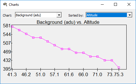
That was Ha, Here is Sii:
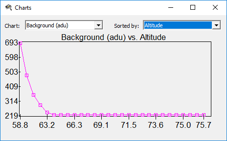
You can see how I set the exposure so the median ADU was above 550 (Gain 75 offset 12) and how it dropped to 219 later in the night.
Set your exposure so that your brightest spots are just below saturation. That will give you the maximum possible dynamic range. The median ADU does not enter the equation. There have been various discussions about gain, noise, tracking, and so forth, however, setting your exposures this way is going to give you the best possible performance from the camera without considering other factors. When you set the exposure lower than this point, you are not using the upper bits of the camera data thus reducing the dynamic range and decreasing the signal to noise ratio.
Well not to start the whole discussion over again, but I’m not in agreement with you on that.
That’s really about higher gain vs. lower gain however but I think there are two tasks in setting exposure:
-
As you say (sort of) not to clip too much, I think you are way too sensitive to any clipping, but in my experience I have some clipping even when working with the next criteria, but when you go at look at WHAT is clipped, it is only the cores of one or two bright stars.
-
expose above the “Noise”, sky glow, read nosie, etc. and I think that’s where the median adu rules of thumb come in.
I guess I can’t help but try to explain my view on dynamic range again. It differs from you because you are assuming (I think) that like in terrestrial photography there is “interesting stuff” all throughout the histogram. In my experience, the “interesting stuff” in deep sky astro imaging is just around or slightly above the right hand side of the hump at the left of the histogram. I think this view is justified by one of the first actions we all take with our data in processing, which is to stretch the data. Taking whatever bits of dynamic range or different tones we have in that small area to the right of the histogram peak and stretching it out so as to cover more dynamic range in the output (while limiting the expansion of the upper parts of the histogram so that stuff is more linear and doesn’t get blown out).
So, how does that lead me to different conclusions about dynamic range and gain? If you turn the gain up, yes your TOTAL dynamic range goes down, BUT if we are only interested in that small area to the right of the histogram peak, increasing the gain means I have more buckets or possible ADU values that small area will be spread across. So it actually means for my target (area of interest), I will have MORE dynamic range, not less, at higher gains.
When I go to stretch, I might be stretching twice or four times as many discrete ADU values, so should also have better post stretch results.
That said, yes, more stars will have their cores clipped. All things in moderation, but I think the higher gains have more application in NB, and in that case the stars have the wrong colors anyway, and I am likely to do tone mapping and replace them with fewer smaller RGB stars from subs with lower gain and shorter (super short) exposures.
1 Like